Model Comparison
finding a good model isn’t always the main problem, sometimes there’re other models that can give better results or we already have many. so comparing models is of big use in such cases.
Here we’re going to apply and compare between some classification machine learning models to get the best one among them.
first we get the spiral data from the kernlab package and plot it
library(kernlab)
data('spirals')
s <- specc(spirals, centers = 2)
spiral_data <- data.frame(x = spirals[,1], y = spirals[,2],
                class = as.factor(s))

library(ggplot2)
ggplot(data = spiral_data) +
  geom_point(aes(x = x, y = y, color = class)) +
  coord_fixed() + theme_bw() +
  scale_color_brewer(palette = 'Set1')
 then we’re going to fit some algorithms on data and compare between them. how accurately they fitted the model, calculating the accuracy of each model and the AUC and visualizing the models.
the algorithms we’ll fit are Logistic Regression, Naive Bayes and Support Vector Machine.
let’s first define a function that gets AUC and the accuracy of each model.
library(ROCR)

accuracy <- function(model, outcome){
  mean(model == outcome)
}

auc <- function(model, outcome) {
  per <- performance(prediction(model, outcome == 2),
                      "auc")
  as.numeric(per@y.values)
}
now we fit the models
# Logistic Regression
logit <- glm(class ~ x + y,
                 family = binomial(link = 'logit'),
                 data = spiral_data)
spiral_data$logit_pred <- ifelse(predict(logit) > 0, 2, 1)
accuracy(spiral_data$logit_pred, spiral_data$class)
## [1] 0.6633333
auc(spiral_data$logit_pred, spiral_data$class)
## [1] 0.6633333
# Naive Bayes
library(e1071)
nb <- naiveBayes(class ~ x + y, data = spiral_data)
spiral_data$nb_pred <- ifelse(
  predict(nb, newdata = spiral_data) == 2, 2, 1)
accuracy(spiral_data$nb_pred, spiral_data$class)
## [1] 0.6533333
auc(spiral_data$nb_pred, spiral_data$class)
## [1] 0.6533333
# SVM
svm_fit <- svm(class ~ x + y, data = spiral_data)
spiral_data$svm_pred <- ifelse(predict(svm_fit) == 2, 2, 1)
accuracy(spiral_data$svm_pred, spiral_data$class)
## [1] 0.6566667
auc(spiral_data$svm_pred, spiral_data$class)
## [1] 0.6566667
Accuracy and AUC can sometimes be equal but they are two different measures …
comparing the models visually on data.
### ON DATA
predictions <- melt(spiral_data, id.vars = c('x', 'y'))
ggplot(predictions, aes(x = x, y = y, color = factor(value))) +
  geom_point() + coord_fixed() +
  scale_colour_brewer(palette = 'Set1') +
  facet_wrap(~ variable) + theme_bw()

seems we don’t have a good model yet. but since the problem is nonlinear, SVM may perform better than the other two with some adjusting to its parameters.
also DECISION TREE or K-NEAREST NEIGHBORS can perform very well in this problem
### decision tree
library(rpart)
tree <- rpart(class ~ x + y, data = spiral_data)
prediction <- predict(tree, newdata = spiral_data, type = 'class')

### knn
library(class)
knn15 <- knn(train = spiral_data[, 1:2], test = spiral_data[, 1:2],
             spiral_data$class, k = 15)
but we will go with Support Vector Machine for now
first we compare between its four kernels to choose the best one of them.
spiral_data <- spiral_data[, 1:3]
# radial
radial <- svm(class ~ x + y, data = spiral_data, kernel = 'radial')
spiral_data$svm_radial <- ifelse(predict(radial) == 2, 2, 1)
# linear
linear <- svm(class ~ x + y, data = spiral_data, kernel = 'linear')
spiral_data$svm_linear <- ifelse(predict(linear) == 2, 2, 1)
# polynomial
polynomial <- svm(class ~ x + y,
                  data = spiral_data, kernel = 'polynomial')
spiral_data$svm_polynomial <- ifelse(predict(polynomial) == 2, 2, 1)
# sigmoid
sigmoid <- svm(class ~ x + y, data = spiral_data, kernel = 'sigmoid')
spiral_data$svm_sigmoid <- ifelse(predict(sigmoid) == 2, 2, 1)

for(i in 4:7){
  print(names(spiral_data)[i])
  print(accuracy(spiral_data[, i], spiral_data$class))
}
## [1] "svm_radial"
## [1] 0.6566667
## [1] "svm_linear"
## [1] 0.66
## [1] "svm_polynomial"
## [1] 0.66
## [1] "svm_sigmoid"
## [1] 0.5566667
### plotting them
predictions <- melt(spiral_data, id.vars = c('x', 'y'))
ggplot(predictions, aes(x = x, y = y, color = factor(value))) +
  geom_point() + coord_fixed() +
  scale_colour_brewer(palette = 'Set1') +
  facet_wrap(~ variable) + theme_bw()

all almost give same results, but we’ll go with the radial kernel tuning its parameters.
tuned_svm_radial <- tune.svm(class ~ x + y, data = spiral_data,
                      kernel = "radial",
                  gamma = seq(0.2, 2, 0.2),
                  cost = c(2 ^ (2:9), 10 ^ (-3:1)))
tuned_svm_radial$best.parameters
##   gamma cost
## 8   1.6    4
spiral_data <- spiral_data[, 1:3]
tuned_model <- svm(class ~ x + y, data = spiral_data,
kernel = 'radial',
gamma = tuned_svm_radial$best.parameters[1],
cost = tuned_svm_radial$best.parameters[2])
spiral_data$tuned_svm <- ifelse(predict(tuned_model) == 2, 2, 1)
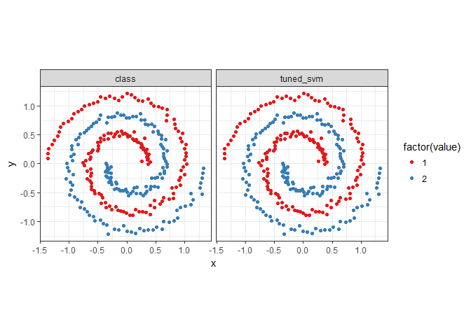
predictions <- melt(spiral_data, id.vars = c('x', 'y'))
ggplot(predictions, aes(x = x, y = y, color = factor(value))) +
geom_point() + coord_fixed() +
scale_colour_brewer(palette = 'Set1') +
facet_wrap(~ variable) + theme_bw()

accuracy(spiral_data$tuned_svm, spiral_data$class)
## [1] 1
auc(spiral_data$tuned_svm, spiral_data$class)
## [1] 1
after comparing so many models, now we have a very fantastic model to use.
Leave a Reply