HousePrice Prediction using R
Fitting a linear model using R’s caret package to predict house prices
Github Link: https://github.com/MNoorFawi/linear-Regression-with-R-and-caret
we first load the train data and the test data without the “id” and “date” columns (the data is already splitted into two datasets “train” and “test” with different extensions)
library(readxl)
house_train <- read.csv("home_data-train .csv",
                        header = FALSE,
                        stringsAsFactors = FALSE)[, -c(1:2)]
house_test <- data.frame(read_excel("HomePrices-Test.xlsx",
                         sheet = "Sheet1"))[, -c(1:2)]
names(house_train) <- names(house_test)
exploring the data
str(house_train)
## 'data.frame':    19998 obs. of  19 variables:
##  $ price        : int  221900 538000 180000 604000 510000 1225000 257500 291850 229500 323000 ...
##  $ bedrooms     : int  3 3 2 4 3 4 3 3 3 3 ...
##  $ bathrooms    : num  1 2.25 1 3 2 4.5 2.25 1.5 1 2.5 ...
##  $ sqft_living  : int  1180 2570 770 1960 1680 5420 1715 1060 1780 1890 ...
##  $ sqft_lot     : int  5650 7242 10000 5000 8080 101930 6819 9711 7470 6560 ...
##  $ floors       : num  1 2 1 1 1 1 2 1 1 2 ...
##  $ waterfront   : int  0 0 0 0 0 0 0 0 0 0 ...
##  $ view         : int  0 0 0 0 0 0 0 0 0 0 ...
##  $ condition    : int  3 3 3 5 3 3 3 3 3 3 ...
##  $ grade        : int  7 7 6 7 8 11 7 7 7 7 ...
##  $ sqft_above   : int  1180 2170 770 1050 1680 3890 1715 1060 1050 1890 ...
##  $ sqft_basement: int  0 400 0 910 0 1530 0 0 730 0 ...
##  $ yr_built     : int  1955 1951 1933 1965 1987 2001 1995 1963 1960 2003 ...
##  $ yr_renovated : int  0 1991 0 0 0 0 0 0 0 0 ...
##  $ zipcode      : int  98178 98125 98028 98136 98074 98053 98003 98198 98146 98038 ...
##  $ lat          : num  47.5 47.7 47.7 47.5 47.6 ...
##  $ long         : num  -122 -122 -122 -122 -122 ...
##  $ sqft_living15: int  1340 1690 2720 1360 1800 4760 2238 1650 1780 2390 ...
##  $ sqft_lot15   : int  5650 7639 8062 5000 7503 101930 6819 9711 8113 7570 ...
plotting the price variable
library(ggplot2)
ggplot(house_train) + geom_density(aes(x = price))

it seems that the price variable distribution is skewed and this indicates that we have to get log(price)
ggplot(house_train) + geom_density(aes(x = log(price)))

we then create a correlation map to know which variables affect the price of a house
library(corrplot)
library(dplyr)
cor_mat <- cor(house_train) %>% round(digits = 2)
corrplot(cor_mat, method = 'number',
         tl.srt = 45, tl.col = 'black')
#method = "shade", type = "upper", shade.col = NA, diag = FALSE

# 2d density plot
#normal geom_point + stat_density2d(aes(color = ..level..), #geom = "raster" / "polygon")

it seems that some variables have weak correlation with the price, so we remove them
unnecessary <- c('sqft_lot', 'condition', 'yr_built', 'yr_renovated',
'zipcode', 'long', 'lat', 'sqft_lot15', 'sqft_basement')

train <- house_train[, -which(names(house_train) %in% unnecessary)]
test <- house_test[, -which(names(house_test) %in% unnecessary)]
then before fitting the model we define functions to extract RSquared and RMSE values from our model. RMSE = root-mean-square error “the lower the better” RSQ = RSquared “the greater the better”
rmse <- function(y, x){
  sqrt(mean((y - x)^2))
}

rsq <- function(y, x) {
  1 - sum((y - x) ^ 2) / sum((y - mean(y)) ^ 2)
}
MODEL FITTING
library(caret)
control <- trainControl(method = "cv", number = 10)
# train the model
model <- train(log(price) ~ ., data = train, method = "lm",
               trControl = control, verbose = FALSE)
exploring model summary
model
## Linear Regression
##
## 19998 samples
##     9 predictor
##
## No pre-processing
## Resampling: Cross-Validated (10 fold)
## Summary of sample sizes: 17999, 17998, 17998, 17998, 17999, 17999, ...
## Resampling results:
##
##   RMSE      Rsquared
##   0.342187  0.5818805
##
## Tuning parameter 'intercept' was held constant at a value of TRUE
##
summary(model)
##
## Call:
## lm(formula = .outcome ~ ., data = dat, verbose = FALSE)
##
## Residuals:
##      Min       1Q   Median       3Q      Max
## -1.67311 -0.24658  0.00735  0.23401  1.31939
##
## Coefficients:
##                 Estimate Std. Error t value Pr(>|t|)
## (Intercept)    1.118e+01  2.190e-02 510.555  < 2e-16 ***
## bedrooms      -6.731e-03  3.267e-03  -2.060   0.0394 *
## bathrooms     -2.098e-02  5.390e-03  -3.892 9.96e-05 ***
## sqft_living    2.761e-04  7.407e-06  37.271  < 2e-16 ***
## floors         6.629e-02  6.383e-03  10.385  < 2e-16 ***
## waterfront     3.543e-01  2.988e-02  11.857  < 2e-16 ***
## view           6.736e-02  3.650e-03  18.456  < 2e-16 ***
## grade          1.716e-01  3.688e-03  46.542  < 2e-16 ***
## sqft_above    -1.494e-04  7.452e-06 -20.048  < 2e-16 ***
## sqft_living15  1.006e-04  6.011e-06  16.732  < 2e-16 ***
## ---
## Signif. codes:  0 '***' 0.001 '**' 0.01 '*' 0.05 '.' 0.1 ' ' 1
##
## Residual standard error: 0.3421 on 19988 degrees of freedom
## Multiple R-squared:  0.5822, Adjusted R-squared:  0.582
## F-statistic:  3094 on 9 and 19988 DF,  p-value: < 2.2e-16
important variables in our model
vimp <- varImp(model)
vimp
## lm variable importance
##
##               Overall
## grade         100.000
## sqft_living    79.160
## sqft_above     40.438
## view           36.860
## sqft_living15  32.985
## waterfront     22.024
## floors         18.715
## bathrooms       4.119
## bedrooms        0.000
plot(vimp)

surprisingly number of bedrooms has no effect at all on the price, meanwhile the grade is the most important variable in the model.
Generalizing the model and getting predictions
we first fit the model over the training data to know how well the model fits the data from which it has been trained.
train$predicted <- predict(model, newdata = train)
cor(log(train$price), train$predicted)
## [1] 0.7629894
rmse(log(train$price), train$predicted)
## [1] 0.3420504
rsq(log(train$price), train$predicted)
## [1] 0.5821528
the model seems to fit the training data well; let’s see how well it can be generalized over the test data that it hasn’t seen yet.
test$predicted <- predict(model, newdata = test)
cor(log(test$price) ,test$predicted)
## [1] 0.8122232
rmse(log(test$price), test$predicted)
## [1] 0.2832296
rsq(log(test$price), test$predicted)
## [1] 0.6496261
the model has even better results over the test data than what it had with the training one. this tells that we have a pretty good model to use over new data
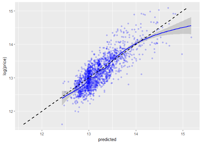
visualizing the predicted vs actual data
to get a sense of how well and close our model fits the data we plot the actual price values as a function of the predicted values with a straight line indicating the ideal relationship it should have and a smoothed one indicating how it actually fits the data.
ggplot(data = test, aes(x = predicted, y = log(price))) +
  geom_point(alpha = 0.2, color = "blue") +
  geom_smooth(aes(x = predicted,
                  y = log(price)), color="blue") +
  geom_line(aes(x = log(price),
                y = log(price)), color = "black",
            linetype = 2, size = 1)
## `geom_smooth()` using method = 'gam'

our model isn’t so far from the ideal one. this is good.
it also good to look at the residuals.
the residual is the difference between the observed value of the dependent variable “log(price)” and the predicted value “predicted” if the points in a residual plot are randomly dispersed around the horizontal axis, a linear regression model is appropriate for the data; otherwise, a non-linear model is more appropriate.
ggplot(data = test, aes(x = predicted,
                      y = predicted - log(price))) +
  geom_point(alpha = 0.2, color = "blue") +
  geom_smooth(aes(x = predicted,
                  y = predicted - log(price)),
              color="black")
## `geom_smooth()` using method = 'gam'

the residuals are pretty randomly dispersed so this means that our model is so fine.
Leave a Reply