Building a clustering algorithm model in R
We will use “Wholesale customers data.csv” at https://archive.ics.uci.edu/ml/machine-learning-databases/00292/ to perform Hierarchical and Kmeans Clustering using R.
Github link for the project and data: https://github.com/MNoorFawi/clustering-with-R
First we load the data and look at it:
data <- read.csv("Wholesale customers data.csv")
str(data)
## 'data.frame':    440 obs. of  8 variables:
##  $ Channel         : int  2 2 2 1 2 2 2 2 1 2 ...
##  $ Region          : int  3 3 3 3 3 3 3 3 3 3 ...
##  $ Fresh           : int  12669 7057 6353 13265 22615 9413 12126 7579 5963 6006 ...
##  $ Milk            : int  9656 9810 8808 1196 5410 8259 3199 4956 3648 11093 ...
##  $ Grocery         : int  7561 9568 7684 4221 7198 5126 6975 9426 6192 18881 ...
##  $ Frozen          : int  214 1762 2405 6404 3915 666 480 1669 425 1159 ...
##  $ Detergents_Paper: int  2674 3293 3516 507 1777 1795 3140 3321 1716 7425 ...
##  $ Delicassen      : int  1338 1776 7844 1788 5185 1451 545 2566 750 2098 ...
summary(data)
##     Channel          Region          Fresh             Milk
##  Min.   :1.000   Min.   :1.000   Min.   :     3   Min.   :   55
##  1st Qu.:1.000   1st Qu.:2.000   1st Qu.:  3128   1st Qu.: 1533
##  Median :1.000   Median :3.000   Median :  8504   Median : 3627
##  Mean   :1.323   Mean   :2.543   Mean   : 12000   Mean   : 5796
##  3rd Qu.:2.000   3rd Qu.:3.000   3rd Qu.: 16934   3rd Qu.: 7190
##  Max.   :2.000   Max.   :3.000   Max.   :112151   Max.   :73498
##     Grocery          Frozen        Detergents_Paper    Delicassen
##  Min.   :    3   Min.   :   25.0   Min.   :    3.0   Min.   :    3.0
##  1st Qu.: 2153   1st Qu.:  742.2   1st Qu.:  256.8   1st Qu.:  408.2
##  Median : 4756   Median : 1526.0   Median :  816.5   Median :  965.5
##  Mean   : 7951   Mean   : 3071.9   Mean   : 2881.5   Mean   : 1524.9
##  3rd Qu.:10656   3rd Qu.: 3554.2   3rd Qu.: 3922.0   3rd Qu.: 1820.2
##  Max.   :92780   Max.   :60869.0   Max.   :40827.0   Max.   :47943.0
Here we can find that except for the first two columns, which can be categories and can be one-hot encoded if needed but we will neglect them here, the rest of the columns are numeric and need to be scaled or normalized. So we scale them and then get the euclidean distance between the observations in order to pass it to the hclust function to do Hierarchical Clustering first …
data[, 1:2] <- apply(data[, 1:2], 2, function(x) as.factor(x))
vars <- colnames(data)

## to one hot encode factor values and normalize numeric ones if needed
# cat <- vars[sapply(data[, vars], class) %in% c("factor", "character")]
num <- vars[sapply(data[, vars], class) %in% c("numeric", "integer")]
# for (i in cat) {
#   dict <- unique(data[, i])
#   for(key in dict){
#     data[[paste0(i, "_", key)]] <- 1.0 * (data[, i] == key)
#  }
# }
# data[, num] <- apply(data[, num], 2, function(x) {
#   (x - min(x)) / (max(x) - min(x))
# })
#
# data <- data[, -which(colnames(data) %in% cat)]
# cmatrix <- as.matrix(sapply(data[, num], as.numeric))

## but here we will only scale numeric values
cmatrix <- scale(data[, num])
head(cmatrix)
##            Fresh        Milk     Grocery     Frozen Detergents_Paper
## [1,]  0.05287300  0.52297247 -0.04106815 -0.5886970      -0.04351919
## [2,] -0.39085706  0.54383861  0.17012470 -0.2698290       0.08630859
## [3,] -0.44652098  0.40807319 -0.02812509 -0.1373793       0.13308016
## [4,]  0.09999758 -0.62331041 -0.39253008  0.6863630      -0.49802132
## [5,]  0.83928412 -0.05233688 -0.07926595  0.1736612      -0.23165413
## [6,] -0.20457266  0.33368675 -0.29729863 -0.4955909      -0.22787885
##       Delicassen
## [1,] -0.06626363
## [2,]  0.08904969
## [3,]  2.24074190
## [4,]  0.09330484
## [5,]  1.29786952
## [6,] -0.02619421
## Hierarchical Clustering
d <- dist(cmatrix, method = "euclidean")
pfit <- hclust(d, method = "ward.D")
plot(pfit, labels = FALSE)

As we can see in the dendrogram plotted, the data can be clustered to different cluster numbers. Hierarchical Clustering with “WARD” method tries to minimize the total within sum of squares (WSS) of the clustering, so based on that, it’s seen in the dendrogram that the data can be clustered to about 4 main clusters. We can see that in the dendrogram with:
plot(pfit, labels = FALSE)
rect.hclust(pfit, k = 4)

To extract the members of each cluster from the hclust object, we can use cutree(). And we can then visualize the data with these clusters.
hcl_groups <- factor(cutree(pfit, k = 4))
## visualize clusters in the data
suppressMessages(library(ggplot2))
data$hcl <- hcl_groups
ggplot(data, aes(x = log(Grocery),
                 y = log(Milk),
                 color = hcl)) +
  geom_point(alpha = 0.7,
             position = position_jitter(h = 0.5, w = 0.5)) +
  theme_minimal() +
  scale_color_brewer(palette = "Set1") +
  labs(x = "Grocery", y = "Milk")

We can clearly see that Milk and Grocery have a linear relationship that is of a strong positive correlation coefficient, so we expect them to be together in one of the clusters.
Bootsrap Evaluation of the Clusters.
Clustering algorithms don’t have an evaluation metric like other supervised algorithms. So it is sometimes hard to tell if the clusters suggested by the algorithm express a real pattern in the data or it is just a random guessing by the algorithm. fpc package has a function which can help in this. clusterboot(), this function does Bootstrap Evaluation to the clusters suggested, i.e. clustering data as usual, then drawing new datasets (of the same size as the original) by resampling the original dataset with replacement then clustering the new dataset. clusterboot() gives two important values; bootmean which measures how stable the cluster is, the more the mean the more stable the cluster is. And bootbrd which tells the number of times the cluster is dissolved or disappered in the process, the less the number, the more stable the cluster is.
## Bootstrap Evaluation of Clusters
suppressMessages(library(fpc))
k_estimated <- 4
cboot_hclust <- clusterboot(cmatrix, clustermethod = hclustCBI,
                            method = "ward.D", k = k_estimated,
                            count = FALSE)
hcl_cboot_groups <- cboot_hclust$result$partition
cboot_hclust$bootmean
## [1] 0.5822147 0.6742406 0.5586298 0.4891219
cboot_hclust$bootbrd
## [1] 29 5 37 58
We can see that cluster two is the most stable among them with and the second most stable one is cluster one. This can tell that other clusters may not be good clusters to cluster the data to. Let’s run another clustering algorithm on the data to see what it will give.
Kmeans Algorithm
Now we will run kmeans algorithm over the dataset but not with the usual kmeans() function, as it requires setting a priori the number of clusters and now we aren’t so sure about it. So we will run the algorithm with another function from fpc again, kmeansruns(). This function has major advantages; we can set a range of Ks and the function will give us the best K according to two different critieria, Calinski Harabasz Index (ch) that measures how separately the clusters are from each others, and Average Silhouette Width (asw) that measures how tightly grouped all the points in the cluster are. So we will be looking for a K value with the greatest number of each one. We will run kmeansruns with both criteria over 10 Ks and compare the output.
## picking K for kmeans
clustering_ch <- kmeansruns(cmatrix, krange = 1:10, criterion = "ch")
clustering_ch$bestk
## [1] 10
clustering_asw <- kmeansruns(cmatrix, krange = 1:10, criterion = "asw")
clustering_asw$bestk
## [1] 2
Ch tells that the best K is 2 while the best K suggested by asw is 10. Let’s plot these values to better explore them.
## plot it
suppressMessages(library(reshape2))
criteria <- data.frame(k = 1:10, ch = scale(clustering_ch$crit),
                       asw = scale(clustering_asw$crit))
criteria <- melt(criteria, id.vars = c("k"),
                  variable.name = "measure",
                  value.name = "score")
ggplot(criteria, aes(x = k, y = score, col = measure)) +
  geom_point(aes(shape = measure)) +
  geom_line(aes(linetype = measure)) +
  scale_x_continuous(breaks = 1:10, labels = 1:10) +
  scale_color_brewer(palette = "Set1") +
  theme_minimal()

Here we can see that at 2 is by far the best value of asw, while with ch, starting from 2 the values are growing after declining a little in 3 but with no big difference. So this can tell that the best number of clusters is 2. N.B. 3 Ks may be also the proper number of K, as cluster 1 and 3 from clusterboot() with hclust were very close in values to each other. N.B. the growing values of ch might tell that the data can be clustered deeper into micro clusters. Here, I will go with 3 just to see where the third cluster might be in the data.
We will run clusterboot again with kmeans and check bootmean and bootbrd.
## clusterboot() revisited with kmeans
kmeans_cboot <- clusterboot(cmatrix, clustermethod = kmeansCBI,
                            runs = 100, iter.max = 100,
                            krange = 3, seed = 13,
                            count = FALSE)
kmeans_cboot_groups <- kmeans_cboot$result$partition
kmeans_cboot$bootmean
## [1] 0.5428560 0.8714325 0.3491429
kmeans_cboot$bootbrd
## [1] 57 0 84
As with hclust, cluster 2 is the most stable and cluster one is the second most stable while cluster 3 is the least. Let’s visualize the clusters together.
We will use Principal Component Analysis (pca) to reduce the dimensions of the dataset into 2 main dimensions in order to visualize it.
## Visualizing Clusters
## PCA done on dimensions you want to examine the clusters on
## those dimensions should be scaled
pca <- prcomp(cmatrix)
visual <- predict(pca, newdata = cmatrix)[, 1:2]
visual <- cbind(as.data.frame(visual),
                cluster = as.factor(kmeans_cboot_groups))
ggplot(visual, aes(x = PC1, y = PC2)) +
  geom_point(aes(col = cluster),
             # position = position_jitter(h = 0.5, w = 0.5),
             alpha = 0.7) +
  theme_minimal() +
    scale_color_brewer(palette = "Set1")

As expected, cluster 1 and 2 are so close to each other, with 2 more densed and grouped together, and cluster 3 are so far away from other clusters and also the points are separated from each other inside the cluster, this is known as other cluster
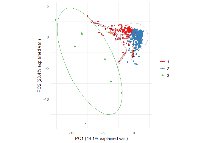
Let’s now visualize the clusters with ggbiplot which gives more expressiveness to the clusters visualization.
suppressMessages(library(ggbiplot))
ggbiplot(pca, obs.scale = 1,
         ellipse = TRUE, circle = TRUE,
         groups = factor(kmeans_cboot_groups)
         ) +
  scale_color_brewer(palette = "Set1", name = "") +
  theme_minimal()

As we expected earlier, Grocery and Milk are together in the same cluster along with Detergents_Paper in cluster 1, while cluster 2 has Delicassen, Fresh and Frozen.
Leave a Reply