Manipulating Large Data with R
Handling large data files with R using chunked and data.table packages.
Here we are going to explore how can we read manipulate and analyse large data files with R.
Github Link: https://github.com/MNoorFawi/handling-big-files-with-R
Getting the data: Here we’ll be using GermanCredit dataset from caret package. It isn’t a very large data but it is good to demonstrate the concepts.
library(caret)
data("GermanCredit")
write.csv(GermanCredit, "german_credit.csv")
Now we have the data file in desk and we want to read it to extract some information from it. We don’t always need to read the whole file, we can go well with subset of the data. For example, for machine learning models we can extract a representable sample from the data to build the model without reading the whole file. That is what we’re going to do here, we will read samples of data to get the information we need without reading the whole file into memory.
We will use the power of chunked package , https://github.com/edwindj/chunked, that enables us to navegate the data files in chunks and do some dplyr manipulations to the data loading only a part of the data in memory making sure that chunk by chunk is processed. chunked is built on top of LaF and uses dplyr syntax.
We will also explore some trick to load the data in chunks with data.table.
N.B. we can also use the command line to do all this. Have a look at https://minimatech.org/data-processing-at-command-line/
Let’s get down to business….
Get a general look at the data
library(chunked)
library(dplyr)
## Here we don't read the file, we just get something like a pointer to it.
data_chunked <- read_chunkwise('german_credit.csv',
                              chunk_size = 100)

data_chunked
# Source: chunked text file 'german_credit.csv' [?? x 63]
#
# # data.frame [6 × 63]
Looking at what data_chunked returns, we get to know the number of columns and it also tells us some information on columns type, for example we have so many integer columns and we have a factor column which is Class.
but what if we want to know the number of rows;
data_chunked %>%
  summarise(n = n()) %>% # chunked will get the number of rows of each chunk
  as.data.frame() %>% # here we read the data returned from summarise()
  summarise(nrows = sum(n)) # and summarise() the length of each chunk

##   nrows
## 1  1000
We saw that there’s a factor variable in the data, so let’s look at its levels’ frequencies in the data;
data_chunked %>%
  group_by(Class) %>%
  summarise(freq = n()) %>%
  as.data.frame() %>%
  group_by(Class) %>%
  summarise(freq = sum(freq))

## # A tibble: 2 x 2
##   Class  freq
##   <fct> <int>
## 1 Good    700
## 2 Bad     300
Fine! let’s do some more complicated query… Imagine we want to know the average age per class of single males who are foreign worker and have less than two credits…
data_chunked %>%
  select(Class, Age,
         Personal.Male.Single,
         ForeignWorker, NumberExistingCredits) %>%
  filter(Personal.Male.Single > 0 &
           ForeignWorker > 0 &
           NumberExistingCredits < 2) %>%
  group_by(Class) %>%
  summarise(mean_age = mean(Age)) %>%
  collect() %>%
  group_by(Class) %>%
  summarise(mean_age = mean(mean_age))

## # A tibble: 2 x 2
##   Class mean_age
##   <fct>    <dbl>
## 1 Good      37.0
## 2 Bad       36.6
As you can see, chunked waits till the last moment to read the data. this is amazing when it comes to big data files.
let’s do some analysis. Let’s plot a scatter plot between Duration and Amount differentiating between them by Class.
library(ggplot2)
data_chunked %>%
  select(Class, Amount, Duration) %>%
  collect() %>%
  ggplot(aes(x = Duration, y = Amount, color = Class)) +
    geom_jitter(alpha = 0.7) +
    scale_color_brewer(palette = 'Set1') +
    theme_minimal() +
    theme(legend.position = 'top')

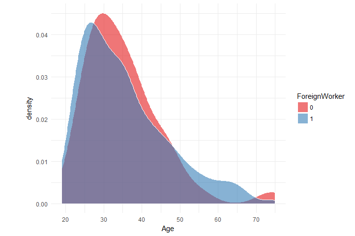
Now what about the distribution of Age per ForeignWorker
data_chunked %>%
  select(Age, ForeignWorker) %>%
  mutate(ForeignWorker = as.factor(ForeignWorker)) %>%
  collect() %>%
  ggplot(aes(x = Age, fill = ForeignWorker)) +
    geom_density(color = 'white', alpha = 0.6) +
    scale_x_continuous(breaks = seq(10, 100, 10)) +
    theme_minimal() + scale_fill_brewer(palette = 'Set1')

GREAT! we have done all this without reading the whole data…
We can also read sample of the data for further analysis.
sampled <- data_chunked %>%
  mutate(rand = runif(100)) %>% ## 100 number of each chunk
  filter(rand < 0.1) %>%
  select(- rand) %>%
  as.data.frame()
dim(sampled)

## [1] 88 63
We can also use sqldf to sample the data.
library(sqldf)
query <- 'SELECT * FROM file ORDER BY RANDOM() LIMIT 100'
df <- read.csv.sql('german_credit.csv',
                   sql = query)
dim(df)

## [1] 100  63
Now we are going to fetch specific rows from data in chunks with data.table. Suppose we only want to do analysis on people with purpose business, so we only need the rows with the “Purpose.Business” columns is TRUE. So first we get the indices of these rows.
indices <- data_chunked %>%
  mutate(n = Purpose.Business > 0) %>%
  select(n) %>%
  collect()
indices <- indices[, 1]
sum(indices)

## [1] 97
Now we can chunk the data with data.table::fread() using run length encoding rle() to get the number of rows which each chunk will read and which it’ll skip.
Here’s what rle is defined in WIKIPEDIA;
Run Length Encoding RLE is a very simple form of lossless data compression in which runs of data (that is, sequences in which the same data value occurs in many consecutive data elements) are stored as a single data value and count, rather than as the original run. This is most useful on data that contains many such runs.
library(data.table)
sequence  <- rle(indices)
index  <- c(0, cumsum(sequence$lengths))[which(sequence$values)] + 1
idx <- data.frame(start = index,
                  length = sequence$length[which(sequence$values)])
head(idx)

##   start length
## 1    12      1
## 2    18      1
## 3    30      2
## 4    34      1
## 5    61      1
## 6    63      2

data_fread <- do.call(
  rbind,
  apply(idx, 1,
              function(x) return(fread(
                "german_credit.csv", nrows = x[2], skip = x[1]))))
dim(data_fread)

## [1] 97 63
N.B. we must define the column names for the resulted data.frame.
We have explored some ways to explore, analyze and sampling large data files without reading all it into memory …
Leave a Reply